Set 3 ARMA

3.1 Operators

3.1.1 Backshift operator

The backshift shift operator (\(\mathbf{B}\)) is an important function in time series analysis, which we define as

\[ \mathbf{B} x_t = x_{t-1} \]

or more generally as

\[ \mathbf{B}^k x_t = x_{t-k} \]

For example, express a random walk, \(x_t = x_{t-1} + w_t\), using \(\mathbf{B}\).

3.1.2 The difference operator

The difference operator (\(\nabla\)) is another important function in time series analysis, which we define as

\[ \nabla x_t = x_t - x_{t-1} \]

For example, what does first-differencing a random walk yield?

The difference operator and the backshift operator are related

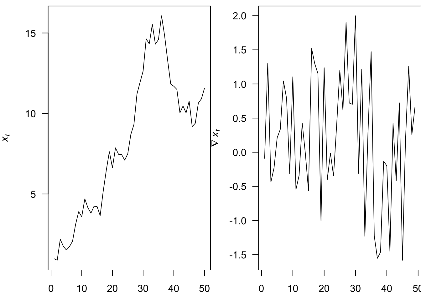
\[ \nabla^k = (1 - \mathbf{B})^k \] Differencing is a simple means for removing a trend

The 1st-difference removes a linear trend

A 2nd-difference will remove a quadratic trend

3.2 Autoregressive (AR) models

An autoregressive model of order p, or AR(p), is defined as

\[x_t = \phi_1 x_{t-1} + \phi_2 x_{t-2} + \dots + \phi_p x_{t-p} + w_t\]

where we assume

1. \(w_t\) is white noise

2. \(\phi_p \neq 0\) for an order-p process

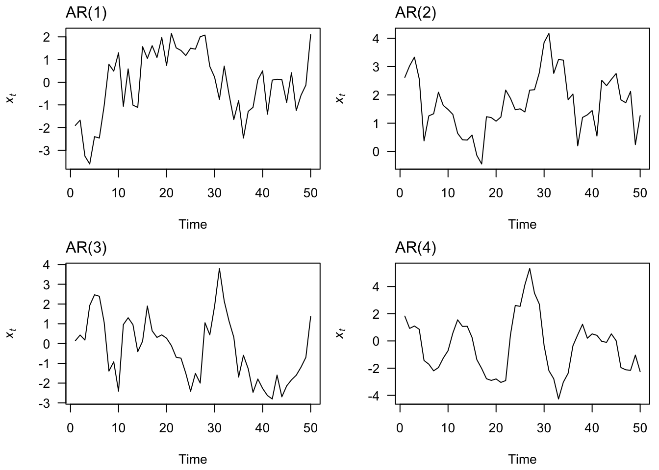
3.2.1 AR(1) Model

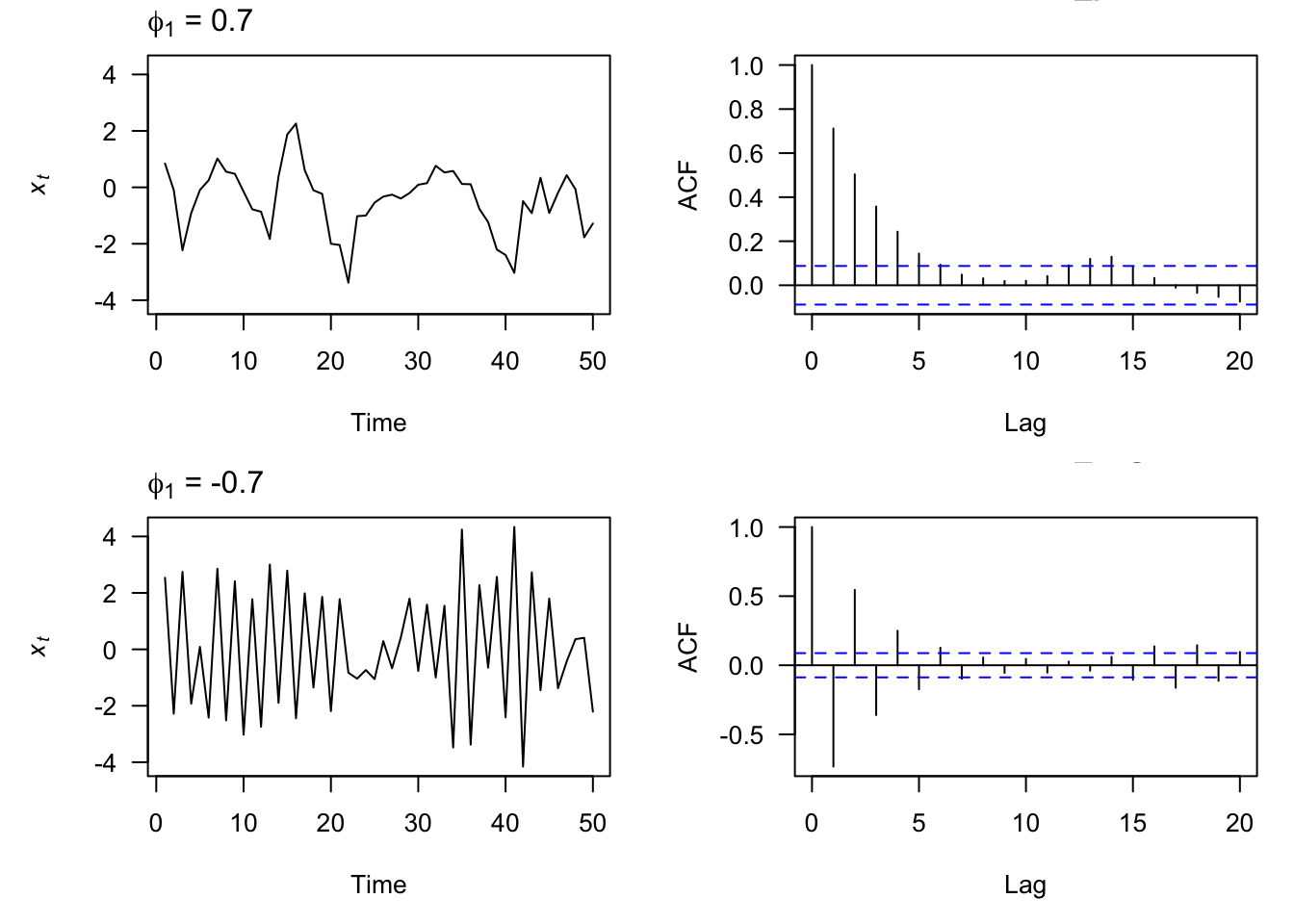
Let’s start by figuring out some properties of the simplest AR model, the AR(1) model:

\[x_t = \phi_0 + \phi_1 x_{t-1} + w_t\]

We start by assuming that \(x_t\) is a stationary time series. Under this assumption, we can show:

\[\begin{align} E(x_t) &= \frac{\phi_0}{1-\phi_1} \\ Var(x_t) &= \frac{\sigma^2_w}{1-\phi_1^2} \\ \rho(h) &= \phi_1^h \end{align}\]

For this to work, \(|\phi_1| < 1\).

3.2.2 Stationarity

We seek a means for identifying whether our AR(p) models are also stationary. We can write out an AR(p) model using the backshift operator:

\[ x_t = \phi_1 x_{t-1} + \phi_2 x_{t-2} + \dots + \phi_p x_{t-p} + w_t \\ \Downarrow \\ \begin{align} x_t - \phi_1 x_{t-1} - \phi_2 x_{t-2} - \dots - \phi_p x_{t-p} &= w_t \\ (1 - \phi_1 \mathbf{B} - \phi_2 \mathbf{B}^2 - \dots - \phi_p \mathbf{B}^p) x_t &= w_t \\ \phi_p (\mathbf{B}^p) x_t &= w_t \\ \end{align} \]

If we treat \(\mathbf{B}\) as a number (or numbers), we can out write the characteristic equation as \(\phi_p (\mathbf{B}^p)\).

To be stationary, all roots of the characteristic equation must exceed 1 in absolute value As a bonus, when this condition is met, then the model is also causal.

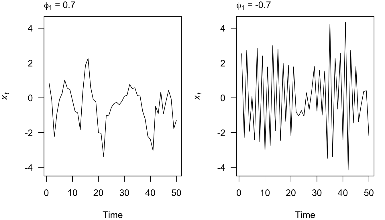
Example, for what value of \(\phi_1\) is AR(1) model stationary?

Are the following AR processes stationary?

1. \(x_t = 0.5 x_{t-1} + w_t\)
2. \(x_t = -0.2 x_{t-1} + 0.4 x_{t-2} + w_t\)
3. \(x_t = x_{t-1} + w_t\)

3.2.3 Autocorrelation

The exponential decay observed in autocorrelation function for the the AR(1) model holds in general for AR(p). This decay may oscillate, as shown below.

3.3 Moving Average (MA) models

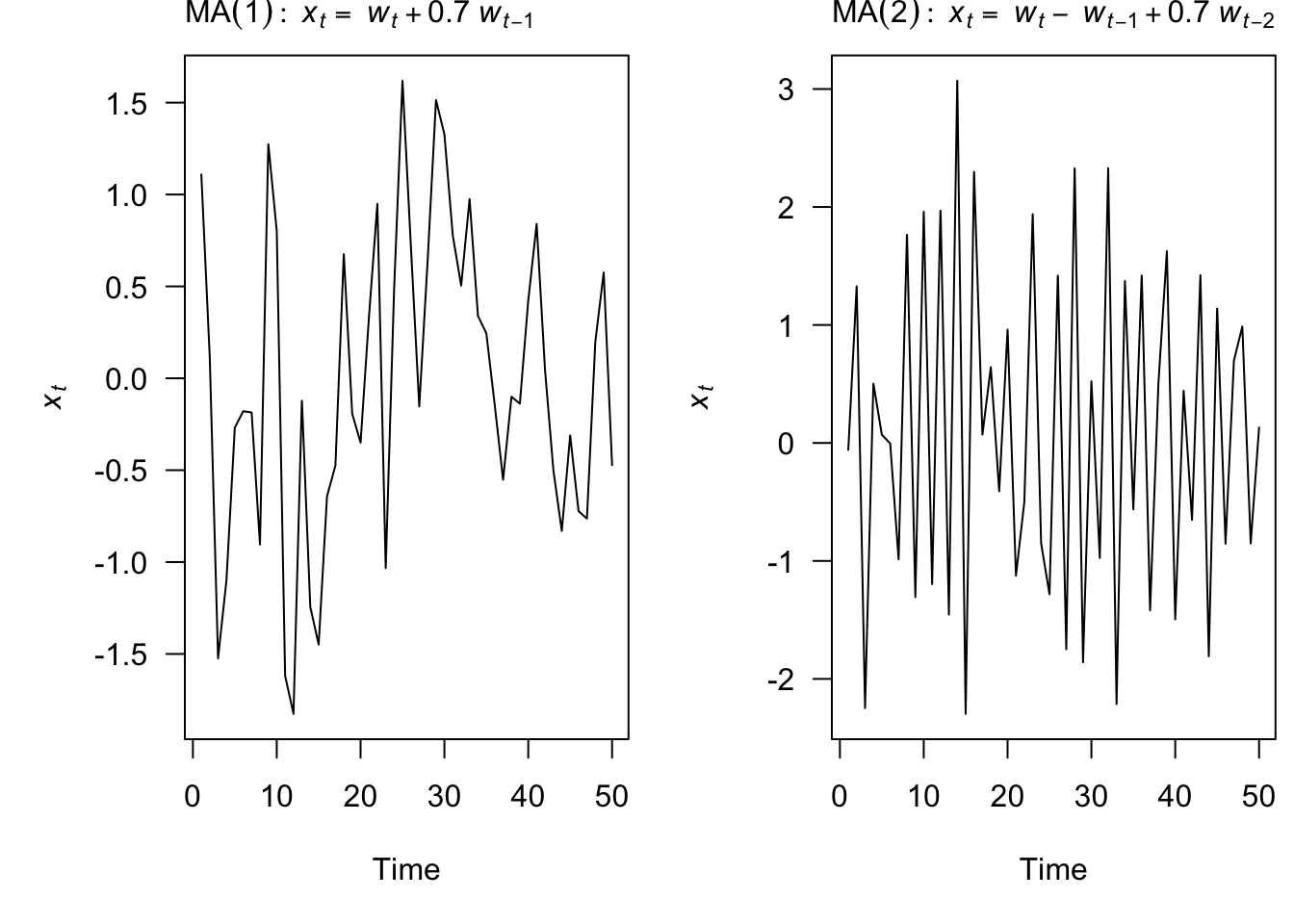
A moving average model of order q, or MA(q), is defined as

\[ x_t = w_t + \theta_1 w_{t-1} + \theta_2 w_{t-2} + \dots + \theta_q w_{t-q}\] where \(w_t\) is white noise

Each of the \(x_t\) is a sum of the most recent error terms

Thus, all MA processes are stationary because they are finite sums of stationary WN processes

3.3.1 Examples of MA(q) models

3.3.2 MA(1) Model

Let’s start by figuring out some properties of the simplest MA model, the MA(1) model:

\[ x_t = \theta_0 + \theta_1 w_{t-1} + w_t \]

We start by assuming that \(x_t\) is a stationary time series. Under this assumption, we can show:

\[\begin{align} E(x_t) &= \theta_0 \\ Var(x_t) &= \sigma^2_w(1+\theta_1^2) \\ \rho(h) &= \frac{\theta_1}{1+\theta_1^2} \text{ for } h=1 \text{ and 0 otherwise. } \end{align}\]

3.3.3 Invertibility

For MA models, we need invertibility in order to identify model paramters. An MA(q) process is invertible if it can be written as a stationary autoregressive process of infinite order without an error term

\[ x_t = w_t + \theta_1 w_{t-1} + \theta_2 w_{t-2} + \dots + \theta_q w_{t-q} \\ \Downarrow ? \\ w_t = x_t + \sum_{k=1}^\infty(-\theta)^k x_{t-k} \]

For example, these MA(1) models are equivalent

\[ x_t = w_t + \frac{1}{5} w_{t-1} ~\text{with} ~w_t \sim ~\text{N}(0,25) \\ \Updownarrow \\ x_t = w_t + 5 w_{t-1} ~\text{with} ~w_t \sim ~\text{N}(0,1) \]

Rewrite an MA(1) model in terms of \(w_t\)

\[ x_t = w_t + \theta w_{t-1} \\ \Downarrow \\ w_t = x_t - \theta w_{t-1} \\ \]

If we constrain \(\lvert \theta \rvert < 1\), then

\[ \lim_{k \to \infty} (-\theta)^{k+1} w_{t-k-1} = 0 \]

and

\[ \begin{align} w_t &= x_t - \theta x_{t-1} - \dots -\theta^k x_{t-k} -\theta^{k+1} w_{t-k-1} \\ w_t &= x_t - \theta x_{t-1} - \dots -\theta^k x_{t-k} \\ w_t &= x_t + \sum_{k=1}^\infty(-\theta)^k x_{t-k} \end{align} \]

3.3.4 Autocorrelation

For the MA(q) model, the autocorrelation function cuts off for \(h >q\). That is,

\[\begin{align} \gamma(h) &= \sigma^2 \sum_{j=0}^{q-h} \theta_j \theta_{j+h}~\text{for }h=0,\ldots,q \\ \gamma(h) &= 0~h>q \end{align}\]

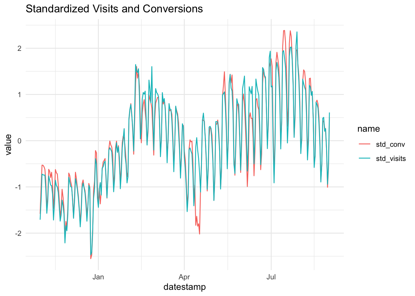
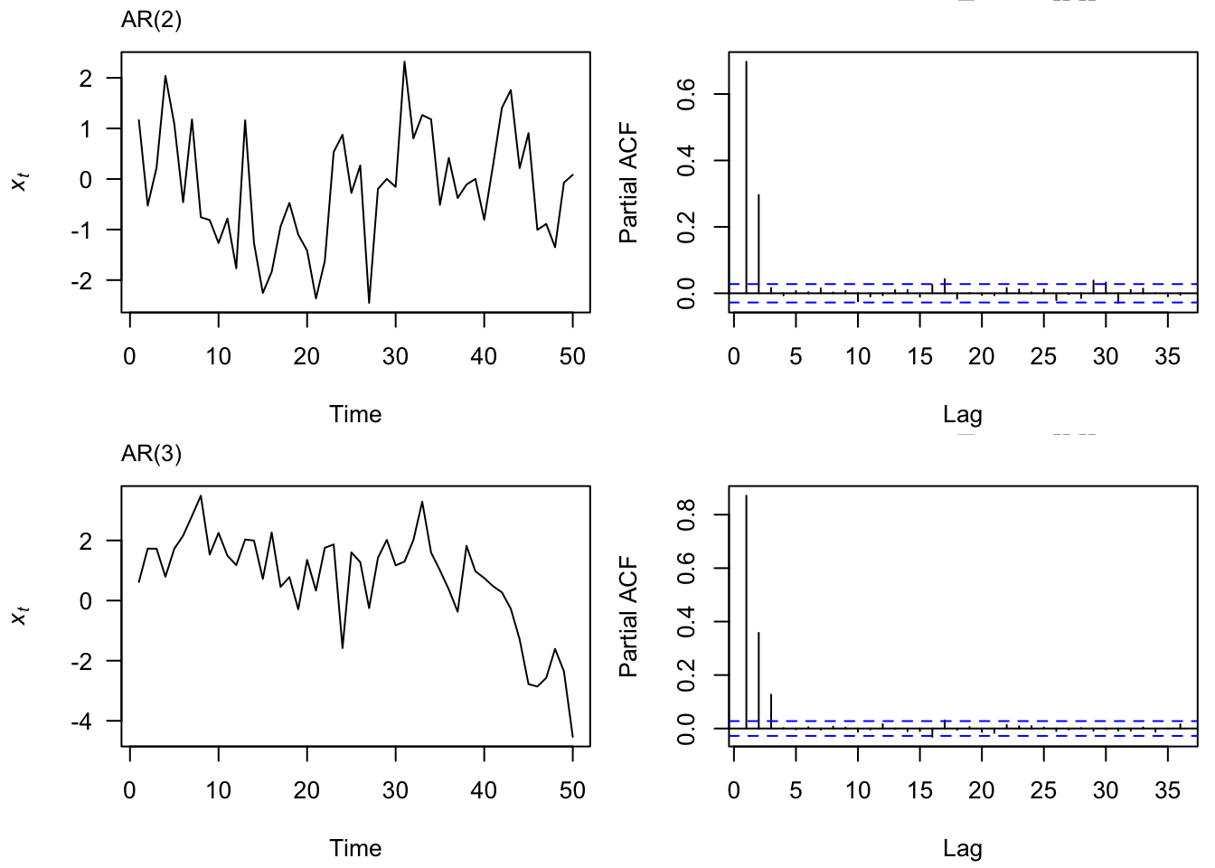
Therefore, the sample ACF is useful for model identification when our data comes from a moving average process, but not so useful for data that comes from an AR process. For this, we introduce the partial autocorrelation (PACF).

3.4 PACF

3.4.1 Definition

The partial autocorrelation of a stationary process, \(x_t\), denoted \(\phi_{hh}\), for \(h=1,2,\ldots\), is

\[\phi_{11}=\text{cor}(x_{t}, x_{t-1}) = \rho_1\] and,

\[\phi_{hh}=\text{cor}(x_{t}-\hat{x}_t, x_{t-h} - \hat{x}_{t-h}),~~h \geq 2\].

The PACF, \(\phi_{hh}\), is the correlation between \(x_t\) and \(x_{t-h}\) with the linear dependence of \(\{x_{t-1}, \ldots, x_{t-h+1} \}\) on each, removed.

3.4.2 AR(1) PACF

Let us calculate \(\phi_{22}\) for the AR(1) model, \(x_t = \phi x_{t-1} + w_t\).

1. Consider the regression of \(x_t\) on \(x_{t-1}\). Choose \(\beta\) to minimize,

\[\begin{align} E(x_t - \beta x_{t-1})^2 &= \gamma(0) - 2\beta \gamma(1) + \beta^2 \gamma(0) \end{align}\]

2. Minimize the expression above to find the estimator of \(\beta\).

3. Plug in this estimated quantity to \(\text{cor}(x_{t}-\hat{x}_{t-1}, x_{t-2} - \hat{x}_{t-2})\)

3.4.3 PACF for AR(p)

For an AR(p) model, when \(h > p\), \(\phi_{hh} = 0\). Thus, the PACF is very informative for model identification when data comes from an autoregressive process.

3.5 AR Estimation

3.5.1 Yule-Walker Equations

Consider the AR(p) model, \(x_t =\)

Now, take the following steps,

1. Multiply both sides by \(x_{t-1}\)
2. Take an expectation
3. This leads to,

\[ \left[ \begin{array}{c} \gamma(1) \\ \vdots \\ \gamma(p) \end{array} \right] = \begin{pmatrix} \gamma(0) & \ldots & \gamma(p-1) \\ \vdots & \ddots & \vdots \\ \gamma(p-1) & \ldots & \gamma(0) \end{pmatrix} \times \left[ \begin{array}{c} \phi_1 \\ \vdots \\ \phi_p \end{array} \right] \] Or, succinctly,

\[\mathbf{\gamma} = \mathbf{\Gamma} \mathbf{\phi}\]

Which can be solved as,

\[\hat{ \mathbf{\phi} } = \mathbf{\Gamma} ^ {-1}\mathbf{\gamma} \] The remaining parameter to be estimated is \(\sigma^2\), the variance of the white noise term. An estimator can be established by multiplying the model by \(x_t\), which leads to

\[\hat{\sigma}^2 = \hat{\gamma}(0) - \sum_{i=1}^{p}\hat{\phi}_i \hat{\gamma}(i)\]

3.5.2 Example

Suppose you aim to estimate \(\mathbf{\phi}\) for a dataset in which \(\hat{\mathbf{\gamma}} = (3.8,3.1,3,2.8)\). What is the Yule-Walker estimate for \(\mathbf{\phi}\) and also for \(\sigma\)?

3.6 ARMA models

An autoregressive moving average, or ARMA(p,q), model is written as

\[ x_t = \phi_1 x_{t-1} + \dots + \phi_p x_{t-p} + w_t + \theta_1 w_{t-1} + \dots + \theta_q w_{t-q} \]

We can write an ARMA(p,q) model using the backshift operator

\[ \phi_p (\mathbf{B}^p) x_t= \theta_q (\mathbf{B}^q) w_t \]

ARMA models are stationary if all roots of \(\phi_p (\mathbf{B}) > 1\)

ARMA models are invertible if all roots of \(\theta_q (\mathbf{B}) > 1\)

3.6.1 \(\psi\) representation

For a causal ARMA\((p,q)\) model, \(\phi_p (\mathbf{B}^p) x_t= \theta_q (\mathbf{B}^q) w_t\), we may write

\[\begin{align} x_t = \sum_{j=0}^\infty \psi_j w_{t-j}. \end{align}\]

Solving for the \(\psi\) weights in general is complicated and can be solved using the ARMAtoMA function in R.

3.6.2 ARMA(1,1)

Solve for the \(\psi\) wieghts in the case of a causal, invertible ARMA(1,1) process.

3.6.3 Forecasting

To forecast with an ARMA model, we simply use the parameter estimates for future periods. For example, consider the following dataset of 500 observations simulated from an ARMA(1,1) process.

set.seed(1)
ex_ts_arma = arima.sim(n = 500, list(ar = c(.8), ma = c(-.3)))
arma_fit = Arima(ex_ts_arma, order = c(1,0,1), include.mean = F)

The fitted model is \(x_t = 0.7732447 x_{t-1} -0.2942922 w_{t-1}\). To forecast two observations in the future, we simply use the parameter estimates as follows:

w_vec = abs( fitted(arma_fit) - ex_ts_arma)
h1 = coefficients(arma_fit)[1] * ex_ts_arma[500] + coefficients(arma_fit)[2] * w_vec[500] # 0.2161869
h2 = coefficients(arma_fit)[1] * h1

Our one step ahead forecast is 0.2161869 and the two step ahead forecast is 0.1671654. The same values can be computed using forecast(arma_fit, h=2)$mean.

3.6.4 Forecast Errors

In order to compute forecast errors, we will make use of the following two parameters:

\[\begin{align} x_{T+h} &= \sum_{j=0}^\infty \psi_j w_{T+h-j} \\ \tilde{x}_{T+h} &= E( x_{T+h} | x_1, \ldots, x_T ) \end{align}\]

Since \(E(w_t | x_1, \ldots, x_T) = w_t\) for \(t \leq T\) and 0 for \(t > T\),

\[\begin{align} x_{T+h} - \tilde{x}_{T+h} &= \sum_{j=0}^{h-1} \psi_j w_{T+h-j} \\ \end{align}\]

Therefore, the variance of this quantity is:

\[\begin{align} \sigma^2 \sum_{j=0}^{h-1} \psi_j ^2 \\ \end{align}\]

With the assumption of normally distributed errors, a 95% prediction interval for \(x_{T+h}\) is,

\[\begin{align} \hat{x}_{T+h} \pm 1.96 \sqrt{ \hat{\sigma}^2_w \sum_{j=0}^{h-1} \psi_j^2 } \end{align}\]

psis = ARMAtoMA(ar = coefficients(arma_fit)[1], ma = coefficients(arma_fit)[2], lag.max = 2)

# confidence interval for one step ahead forecast
c(h1 - qnorm(.975) * sqrt( arma_fit$sigma2 ) , h1 + qnorm(.975) * sqrt ( arma_fit$sigma2 )) # (-1.8, 2.2)

# confidence interval for 2 step ahead forecast
h2_se = sqrt( arma_fit$sigma2 * (1 + psis[1]^2 ) )
c(h2 - qnorm(.975) * h2_se, h2 + qnorm(.975) * h2_se) # (-2.0, 2.4)

Or, use forecast(arma_fit, h = 2)

3.7 Lab 2

1. Simulate data from an AR(1) process in which \(\phi_1 = 0.6\). For sample sizes \(n=10,10^3,10^5\), plot the difference between the theoretical autocorrelation and the observed (sample) autocorrelation for lags 1 through 20. What do you observe?

2. Simulate data from the MA(3) model: \(x_t = w_t+\theta_1w_{t-1}+\theta_2w_{t-2}+\theta_3w_{t-3}\) in which \(\theta = (0.7,0.6,0.2)\). For sample sizes \(n=10,10^3,10^5\), plot the difference between the theoretical autocorrelation and the observed (sample) autocorrelation for lags 1 through 20. What do you observe?

3. For an MA(1), \(x_t = w_t + \theta w_{t-1}\) with \(|\theta|<1\), derive an expression for \(\phi_{22}\). Simulate data from this process and plot the difference between the theoretical value of \(\phi_{22}\) and the sample quantity (which you can compute using pacf).

4. Using ACF & PACF for model ID

Model	ACF	PACF
AR(p)	Tails off slowly	Cuts off after lag p
MA(q)	Cuts off after lag q	Tails off slowly
ARMA(p,q)	Tails off slowly	Tails off slowly

5. Suppose you aim to estimate \(\mathbf{\phi}\) for an AR(2) model in which \(\hat{\mathbf{\gamma}} = (2.1,1.5,1.3)\). What is the Yule-Walker estimate for \(\mathbf{\phi}\) and also for \(\sigma\)?

6. Set up the likelihood function for and AR(p) model