Set 4 ARIMA Models
4.1 AR Models
An autoregressive model of order p, or AR(p), is defined as
\[ x_t = \phi_0 + \phi_1 x_{t-1} + \phi_2 x_{t-2} + \dots + \phi_p x_{t-p} + w_t \]
where we assume
\(w_t\) is white noise. That is, \(w_t \sim N(0,\sigma^2_w)\).
\(\phi_p \neq 0\) for an order-p process
4.1.1 AR(1) Model
Let’s start by figuring out some properties of the simplest AR model, the AR(1) model:
\[ x_t = \phi_0 + \phi_1 x_{t-1} + w_t \]
We start by assuming that \(x_t\) is a stationary time series. Under this assumption, we can show:
\[\begin{align} E(x_t) &= \frac{\phi_0}{1-\phi_1} \\ Var(x_t) &= \frac{\sigma^2_w}{1-\phi_1^2} \\ \rho(h) &= \phi_1^h \end{align}\]
For this to work, \(|\phi_1| < 1\). Now let’s simulate some data from an AR1 model and compare theoretical and observed quantities.
set.seed(1)
phi_1 = 0.5
sigsq_w = 1
x = arima.sim(n = 10000, model = list(ar=c(phi_1)), sd = sigsq_w)| quantity | theory | empirical |
|---|---|---|
| mean | 0.000000 | -0.0142169 |
| variance | 1.333333 | 1.3889404 |
| ACF, k=2 | 0.250000 | 0.2611053 |
4.1.2 AR Stationarity
In the case of the AR(1) model, it was apparent that the condition we needed to ensure a stationary model was the condition that \(|\phi_1| < 1\). For the general AR(p) model, though, the condition is more complicated. Before defining the condition, we define the backshift operator, \(\mathbf{B}\):
\[\mathbf{B}x_t = x_{t-1}\].
Using this operator, we can re-write the AR(p) model as,
\[ x_t = \phi_1 x_{t-1} + \phi_2 x_{t-2} + \dots + \phi_p x_{t-p} + w_t \\ \Downarrow \\ \begin{align} x_t - \phi_1 x_{t-1} - \phi_2 x_{t-2} - \dots - \phi_p x_{t-p} &= w_t \\ (1 - \phi_1 \mathbf{B} - \phi_2 \mathbf{B}^2 - \dots - \phi_p \mathbf{B}^p) x_t &= w_t \\ \phi_p (\mathbf{B}^p) x_t &= w_t \\ \end{align} \]
We will refer to \(\phi_p (\mathbf{B}^p)\) as the characteristic equation. To be stationary, all roots of the characteristic equation must exceed 1 in absolute value. To make this more concrete, let’s go through some examples.
- \(x_t = 0.5 x_{t-1} + w_t\)
- \(x_t = -0.2 x_{t-1} + 0.4 x_{t-2} + w_t\)
- \(x_t = x_{t-1} + w_t\)
4.2 MA Models
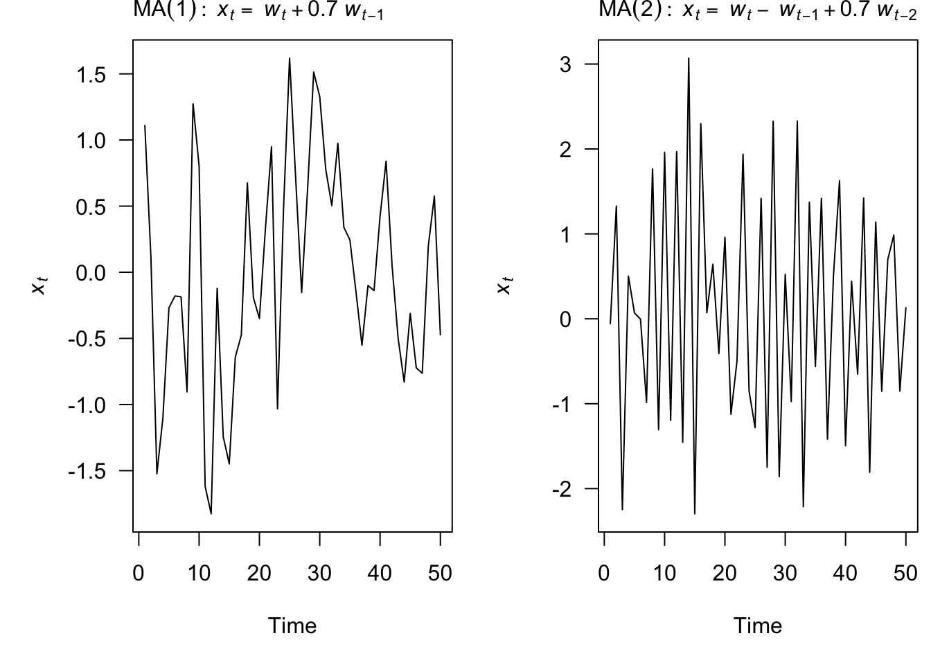
A moving average model of order q, or MA(q), is defined as
\[ x_t = \theta_0 + w_t + \theta_1 w_{t-1} + \theta_2 w_{t-2} + \dots + \theta_q w_{t-q} \] where \(w_t\) is white noise
Each of the \(x_t\) is a sum of the most recent error terms
Thus, all MA processes are stationary because they are finite sums of stationary WN processes.
4.2.1 MA(1) Model
Let’s start by figuring out some properties of the simplest MA model, the MA(1) model:
\[ x_t = \theta_0 + \theta_1 w_{t-1} + w_t \]
We start by assuming that \(x_t\) is a stationary time series. Under this assumption, we can show:
\[\begin{align} E(x_t) &= \theta_0 \\ Var(x_t) &= \sigma^2_w(1+\theta_1^2) \\ \rho(h) &= \frac{\theta_1}{1+\theta_1^2} \text{ for } h=1 \text{ and 0 otherwise. } \end{align}\]
Now let’s simulate some data from an MA1 model and compare theoretical and observed quantities.
set.seed(1)
theta_1 = 0.5
sigsq_w = 1
z = arima.sim(n = 10000, model = list(ma=c(theta_1)), sd = sigsq_w)| quantity | theory | empirical |
|---|---|---|
| mean | 0.00 | -0.0098233 |
| variance | 1.25 | 1.2937915 |
| ACF, k=2 | 0.40 | 0.4124200 |
4.3 ARMA Models
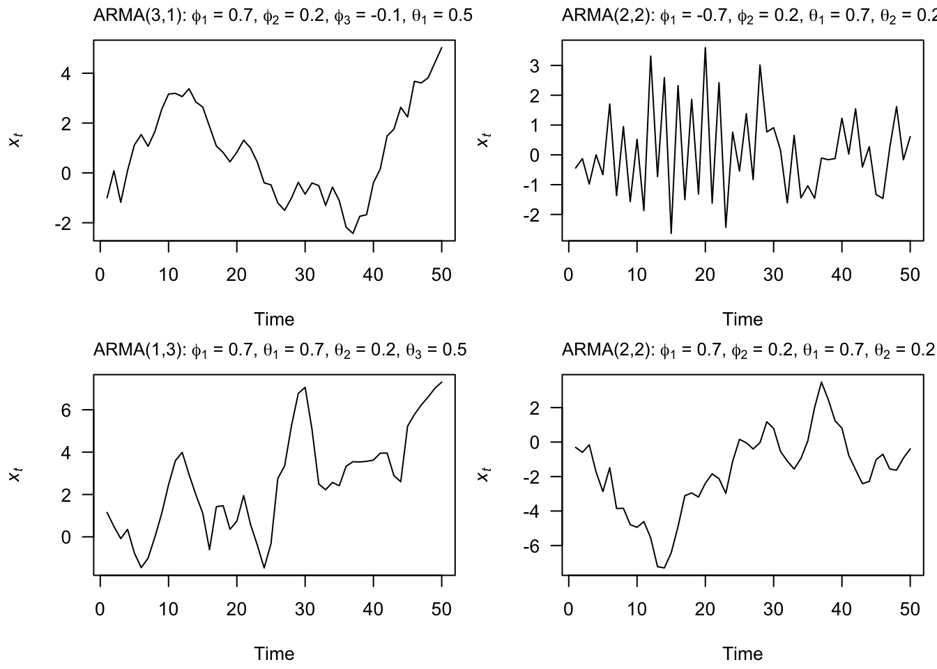
An autoregressive moving average, or ARMA(p,q), model is written as
\[ x_t = \phi_1 x_{t-1} + \dots + \phi_p x_{t-p} + w_t + \theta_1 w_{t-1} + \dots + \theta_q w_{t-q} \]
4.4 ARIMA Models
Our data is not always stationary. If the data do not appear stationary, differencing can help. This leads to the class of autoregressive integrated moving average (ARIMA) models. ARIMA models are indexed with orders (p,d,q) where d indicates the order of differencing.
\(\{x_t\}\) follows an ARIMA(p,d,q) process if \((1-\mathbf{B})^d x_t\) is an ARMA(p,q) process.
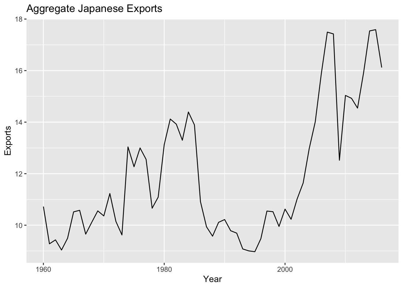
For example, if we look at Japan exports over the time period from 1960 to 2016, we see a clear evolution in the mean of the time series, indicating that the time series is not stationary.
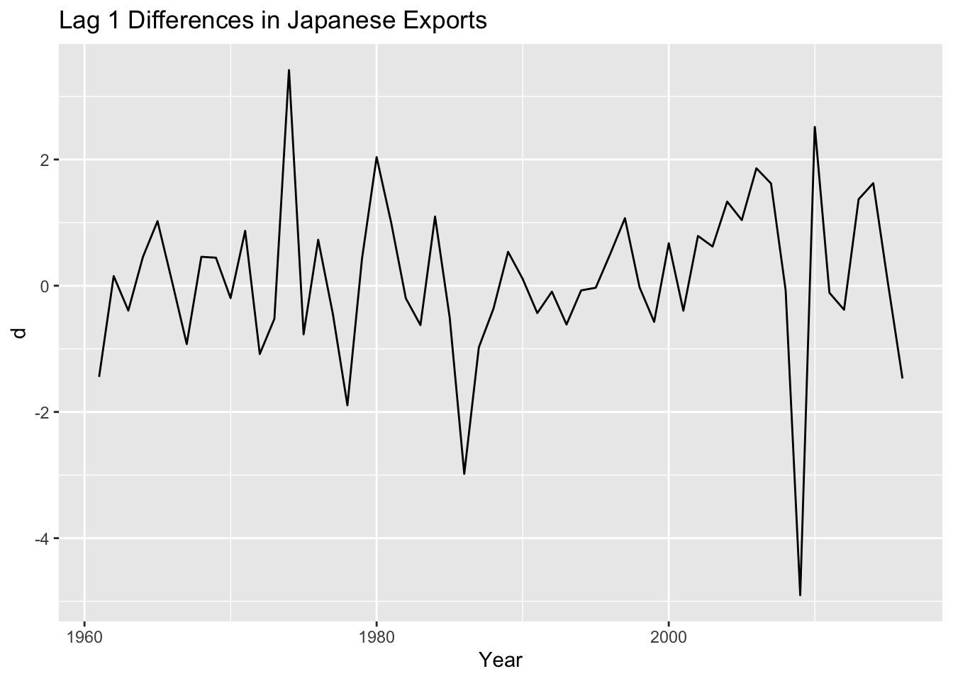
As we saw in week one, if we instead look at the year over year changes in exports, we see something that more closely resembles a stationary time series.
4.4.1 Model Selection/ Fitting
The general sequence of steps involved in fitting an ARIMA model to a given time series are:
- Evaluate whether the time series is stationary
- If not, make it stationary - select the differencing level (d)
- Select the AR level (p) and the MA level (q) that optimize the AIC
Steps two and three are automated with the function forecast::auto.arima function. For instance,
## Series: je$Exports
## ARIMA(0,1,0)
##
## sigma^2 = 1.628:  log likelihood = -93.1
## AIC=188.21   AICc=188.28   BIC=190.24
##
## Training set error measures:
##                     ME     RMSE      MAE       MPE     MAPE      MASE
## Training set 0.0948585 1.264655 0.883942 0.2186117 7.269751 0.9826653
##                     ACF1
## Training set -0.04317139
4.4.2 Model Checking
4.4.2.1 Check the residuals
Residuals = difference between the observations (data), \(y\), and expected (fitted) values, \(\hat{y}\). Thus, the i’th residual is: \(y_i-\hat{y}_i\).
In R, we can obtain the vector of residuals using the residuals function, as shown below.
4.4.2.2 residuals() function in R
The residuals() function will return the residuals for fitted models.
## Time Series:
## Start = 1
## End = 57
## Frequency = 1
##  [1]  0.01072294 -1.44501952  0.15303390 -0.39309669  0.45625211  1.02356255
##  [7]  0.06053730 -0.92437932  0.45807416  0.44426518 -0.19594755  0.86880508
## [13] -1.08192227 -0.52480724  3.41625812 -0.76990990  0.72818035 -0.44252813
## [19] -1.89419993  0.42955074  2.03742971  0.99396401 -0.20034080 -0.62338421
## [25]  1.09590411 -0.50007152 -2.98081554 -0.97493052 -0.36290393  0.53728879
## [31]  0.10797014 -0.43368768 -0.09399316 -0.61422391 -0.07420507 -0.03185334
## [37]  0.50727239  1.06978245 -0.02437143 -0.57272023  0.67272500 -0.39538586
## [43]  0.78912188  0.62107244  1.33273884  1.04040881  1.86046117  1.62041428
## [49] -0.06927885 -4.90312357  2.51584283 -0.11176077 -0.38024365  1.37064557
## [55]  1.62490343  0.04862657 -1.46977556
To check the fit of our model, we want to check that the residuals are white noise.
4.4.3 Forecasting
4.4.3.1 Point Estimates
The basic idea of forecasting with an ARIMA model is to estimate the parameters and forecast forward.
For example, let’s say we want to forecast with a ARIMA(2,1,0) model with drift: \[z_t = \mu + \beta_1 z_{t-1} + \beta_2 z_{t-2} + e_t\] where \(z_t = x_t - x_{t-1}\), the first difference.
Arima() would write this model:
\[(z_t-m) = \beta_1 (z_{t-1}-m) + \beta_2 (z_{t-2}-m) + e_t\] The relationship between \(\mu\) and \(m\) is \(\mu = m(1 - \beta_1 - \beta_2)\).
Let’s estimate the \(\beta\)’s for this model from Japan export.
##         ar1         ar2       drift
## -0.05580519 -0.18850080  0.10736838
## drift
## 0.1335991So we can forecast with this model:
\[z_t = 0.1335991 -0.05580519 z_{t-1} - 0.18850080 z_{t-2} + e_t\] To obtain the \(T+1\) forecast value:
zt_1 = 16.119153 - 17.588928
zt_2 = 17.588928 - 17.540302

16.119153 + (0.1335991 - 0.05580519 * zt_1 - 0.18850080 * zt_2)
## [1] 16.325614.4.3.2 Standard Errors
To obtain the standard errors of the model forecast, it is helpful to reformulate the ARIMA model as an infinite order MA model. Any ARIMA model can be written as an infinite order MA model:
\[\begin{align} x_t - \mu &= w_t + \psi_1 w_{t-1} + \psi_2 w_{t-1} + \ldots + \psi_k w_{t-k} + \ldots \\ &= \sum_{j=0}^\infty \psi_j w_{t-j} \text{ where } \psi_0=1 \end{align}\]
For example, the AR(1) model:
\[\begin{align} y_t &= \phi y_{t-1} + w_t \\ &= \phi ( \phi y_{t-1} + w_{t-1} ) + w_t \\ &= \phi^2 y_{t-1} + \phi w_{t-1} + w_t \\ &= \sum_{j=0}^{\infty} \phi^j w_{t-j} \end{align}\]
The standard deviation of the forecast error at time \(T+h\) is,
\[\begin{align} \sqrt{ \hat{\sigma}^2_w \sum_{j=0}^{h-1} \psi_j^2 } \end{align}\]
With the assumption of normally distributed errors, a 95% prediction interval for \(x_{T+h}\) is,
\[\begin{align} \hat{x}_{T+h} \pm 1.96 \sqrt{ \hat{\sigma}^2_w \sum_{j=0}^{h-1} \psi_j^2 } \end{align}\]
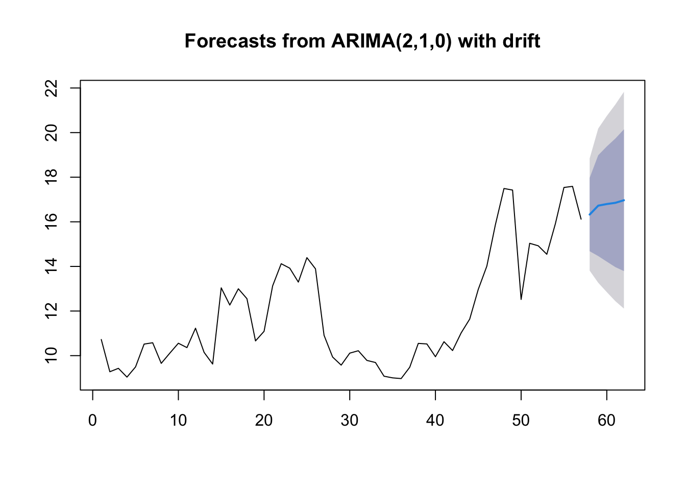
For example, the one step ahead forecast for the Japan Export model has a 95% prediction interval:
## [1] 13.81181 18.83941You can also use the forecast function to obtain point estimates and prediction intervals. For example,
4.5 Lab 3
- Fill in the question marks in the table below. Additionally, for each box in the table, provide empirical evidence of the table entry using simulated data. For example, simulate data (you can use
arima.simor write your own code) that follows a AR(p) process to show that the ACF tails off slowly.
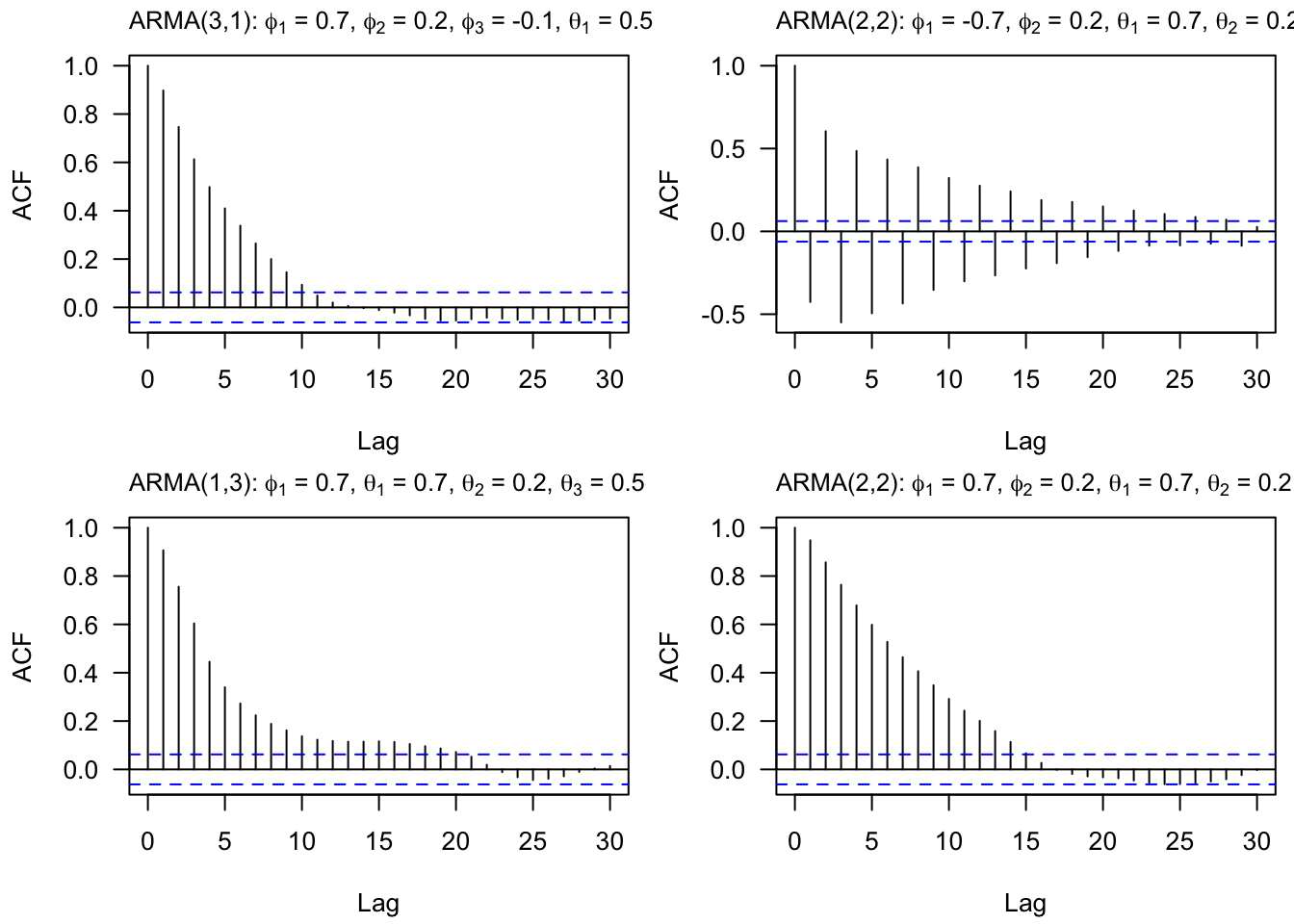
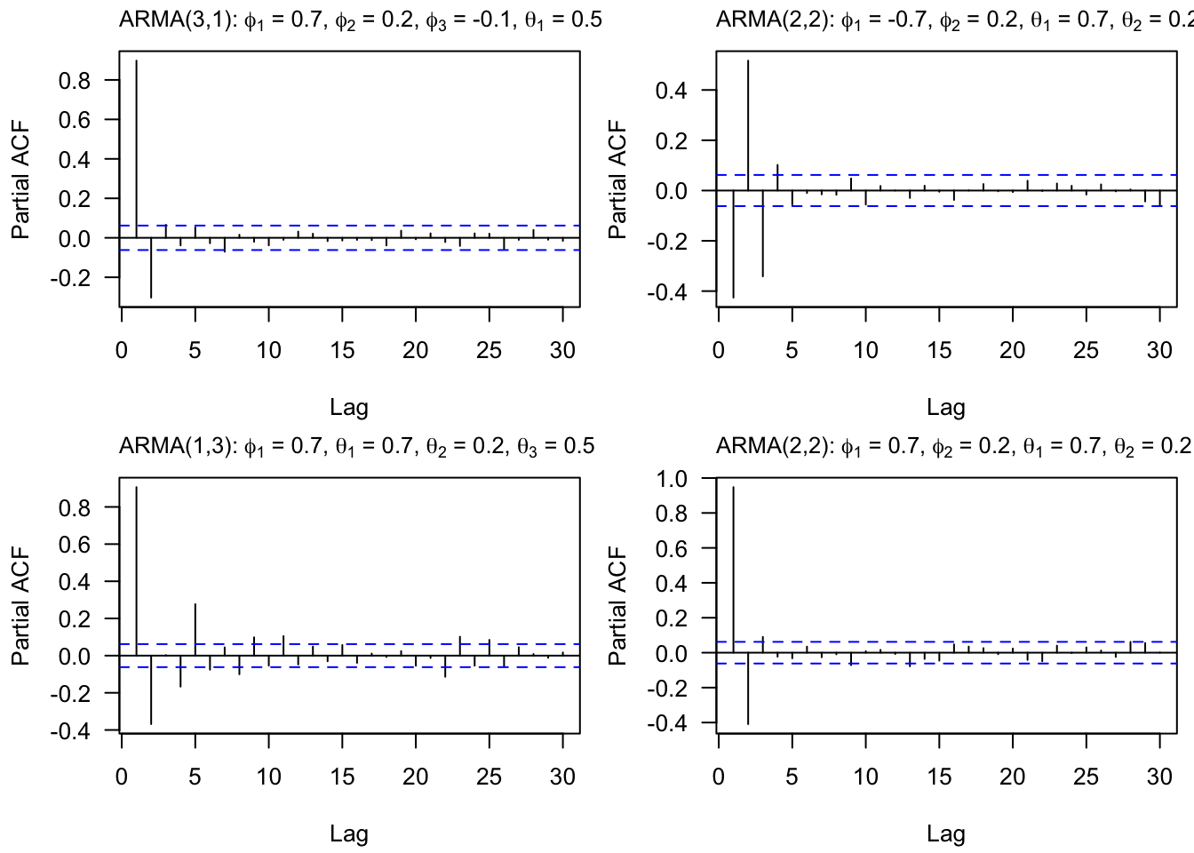
| Model | ACF | PACF |
|---|---|---|
| AR(p) | Tails off slowly | Cuts off after lag ? |
| MA(q) | Cuts off after lag ? | Tails off slowly |
| ARMA(p,q) | Tails off slowly | Tails off slowly |
- Consider
fpp3::aus_airpassengers, the total number of passengers (in millions) from Australian air carriers for the period 1970-2011.
- Use
forecast::auto.arima()to find an appropriate ARIMA model. What model was selected? Write the model in terms of the backshift operator. - Check that the residuals look like white noise.
- Plot forecasts for the next 10 periods.
- Plot forecasts from an ARIMA(0,1,0) model with drift and compare these to the automatically selected model.
- Choose an employment type from
fpp3::us_employment, the total employment in different industries in the United States.
- Are the data stationary? If not, find an appropriate transformation which yields stationary data.
- Examine ACF and PACF plots of the transformed data (if this was necessary to attain stationarity) to identify a couple of ARIMA models that might be useful in describing the time series. Which of your models is the best according to their AIC values?
- Estimate the parameters of your best model and do diagnostic testing on the residuals. Do the residuals resemble white noise? If not, try to find another ARIMA model which fits better.
- Forecast the next 3 years of data. Get the latest figures from https://fred.stlouisfed.org/categories/11 to check the accuracy of your forecasts.
- Eventually, the prediction intervals are so wide that the forecasts are not particularly useful. How many years of forecasts do you think are sufficiently accurate to be usable?
4.6 Lab 3.5
Another way that a time series may violate stationarity is with seasonality. For example, the Leisure and Hospitality sector of the economy spikes in the summer and dips in the winter months. We will look at employment (in thousands) in this sector since 2010:
leisure = fpp3::us_employment %>%
  filter(Title == "Leisure and Hospitality", year(Month) >= 2010) %>%
  select(Month, Employed)
Make a plot of this time series and comment on the trend and the seasonality.
Find appropriate transformation(s) to make the time series stationary. What were the transformations? Provide any necessary plots to validate stationarity.
Use
auto.arimato fit an ARIMA model to the data. You can use either the original time series or the transformed time series. In either case, you may find it helpful to coerce your input time series into a time series object with frequency 12. This will ensure that the function explores seasonal parameters and transformations in the fitting process. What model was selected?Use
forecastto forecast the next twelve months of data. Plot the forecast along with the orginal time series. Does the model capture the trend and seasonality?
