Set 6 Covariates
For this chapter, we will look at modelling the amount of quotes generated by an insurance company using TV advertising spend as a predictor. The dataset is contained in fpp3::insurance. This chapter requires the following packages: fpp3 (for the insurance dataset), forecast (for auto.arima), dynlm (dynamic linear model), bsts (Bayesian Structural Time series).
insurance %>% pivot_longer(-Month) %>%
  ggplot(aes(x = Month, y = value)) +
  geom_line(aes(color = name)) +
  theme_minimal() + ggtitle("Advertising verus Quotes")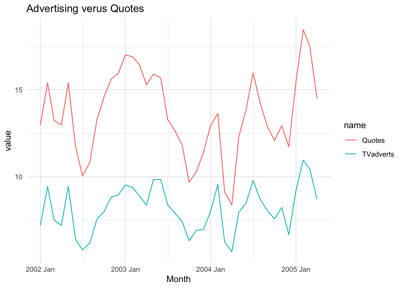
6.1 Linear Regression
We begin by modeling \(y=\) Quotes as a linear function of \(x=\) TV Spend. That is, we have the following model:
\[\begin{align} y_t = \beta_0 + \beta_1 x_t + e_t, \end{align}\]
where \(e_1, \ldots, e_t\) are mutually independent and each \(e_t \sim \text{N}(0,\sigma^2)\).
# option one - simple linear regression
linmod = lm(Quotes ~ TVadverts, data = insurance)
linmod %>% tidy %>% kable()| term | estimate | std.error | statistic | p.value |
|---|---|---|---|---|
| (Intercept) | -0.2401883 | 0.9008432 | -0.2666261 | 0.7911986 |
| TVadverts | 1.6934377 | 0.1088208 | 15.5617088 | 0.0000000 |
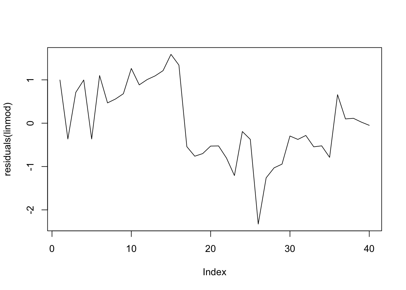
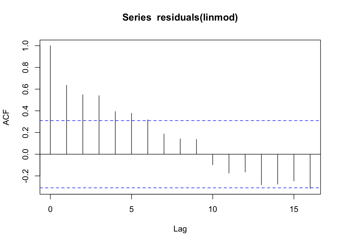
When we do regressions using time series variables, it is common for the errors (residuals) to have a time series structure. This violates the usual assumption of independent errors made in ordinary least squares regression. The consequence is that the estimates of coefficients and their standard errors will be wrong if the time series structure of the errors is ignored.
6.2 dynlm Linear Model
Another way of fitting a linear model to time series data is using the package dynlm. This package, through its namesake function dynlm, fits the same model as above but is noteworthy for its helpful set of functions related to time. Before showing those, let us fit the same model as above using dynlm.
# option two - time series regression: LM with very useful time functions
y = ts(insurance$Quotes, frequency = 4)
x1 = ts(insurance$TVadverts, frequency = 4)
md = dynlm(y ~ x1 )
summary(md) %>% tidy() %>% kable()| term | estimate | std.error | statistic | p.value |
|---|---|---|---|---|
| (Intercept) | -0.2401883 | 0.9008432 | -0.2666261 | 0.7911986 |
| x1 | 1.6934377 | 0.1088208 | 15.5617088 | 0.0000000 |
The results from this model are identcal to the simple linear regression. The utility of this package comes from the ease with which you can add lagged terms, trends and seasonal factors:
6.3 lm with ARIMA Errors
See this site for additional information.
It is possible to adjust estimated regression coefficients and standard errors when the errors have an ARIMA structure. The purpose is to adjust “ordinary” regression estimates for the fact that the residuals have an ARIMA structure.
In this case, the model is written as,
\[\begin{align} y_t &= \beta_0 + \beta_1 x_t + \eta_t \\ \eta_t &= \phi_1 \eta_{t-1} + \dots + \phi_p \eta_{t-p} + w_t + \theta_1 w_{t-1} + \dots + \theta_q w_{t-q}, \end{align}\]
where \(w_t \sim N(0, \sigma^2)\) are white noise. This model can be fit within auto.arima or Arima.
# option three - time series with ARIMA errors
linmod2 = auto.arima(insurance$Quotes, xreg = as.matrix(insurance$TVadverts))
summary(linmod2)
## Series: insurance$Quotes
## Regression with ARIMA(0,1,0) errors
##
## Coefficients:
## xreg
## 1.3485
## s.e. 0.0666
##
## sigma^2 = 0.3301: log likelihood = -33.22
## AIC=70.44 AICc=70.77 BIC=73.77
##
## Training set error measures:
## ME RMSE MAE MPE MAPE MASE
## Training set -0.01299736 0.5599955 0.4354811 -0.09980506 3.271638 0.2767685
## ACF1
## Training set 0.1664547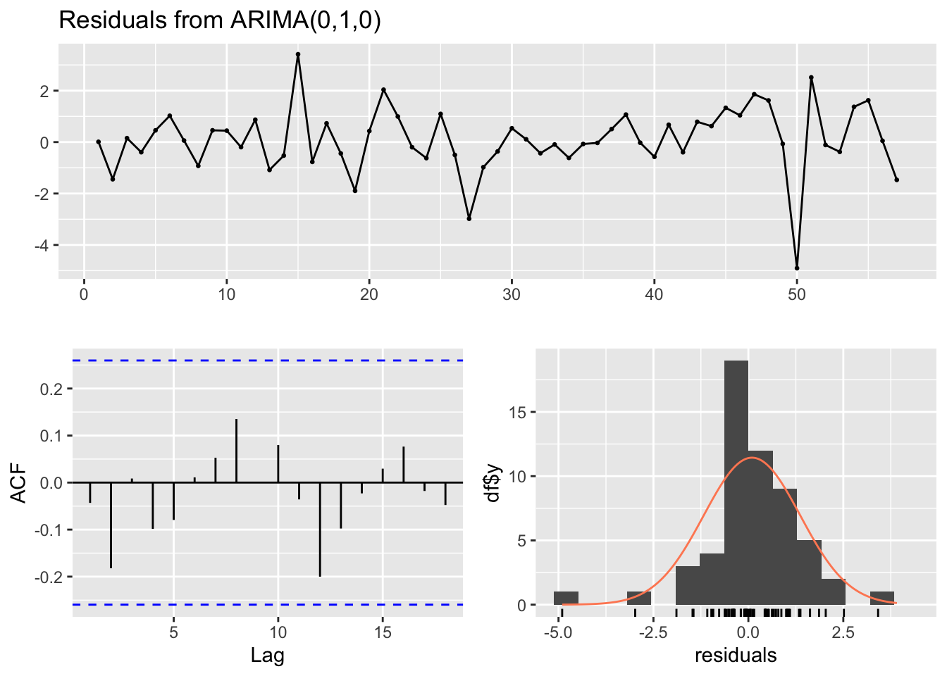
##
##  Ljung-Box test
##
## data:  Residuals from ARIMA(0,1,0)
## Q* = 5.0746, df = 10, p-value = 0.8861
##
## Model df: 0.   Total lags used: 10
6.4 State Space Model
6.4.1 Framework
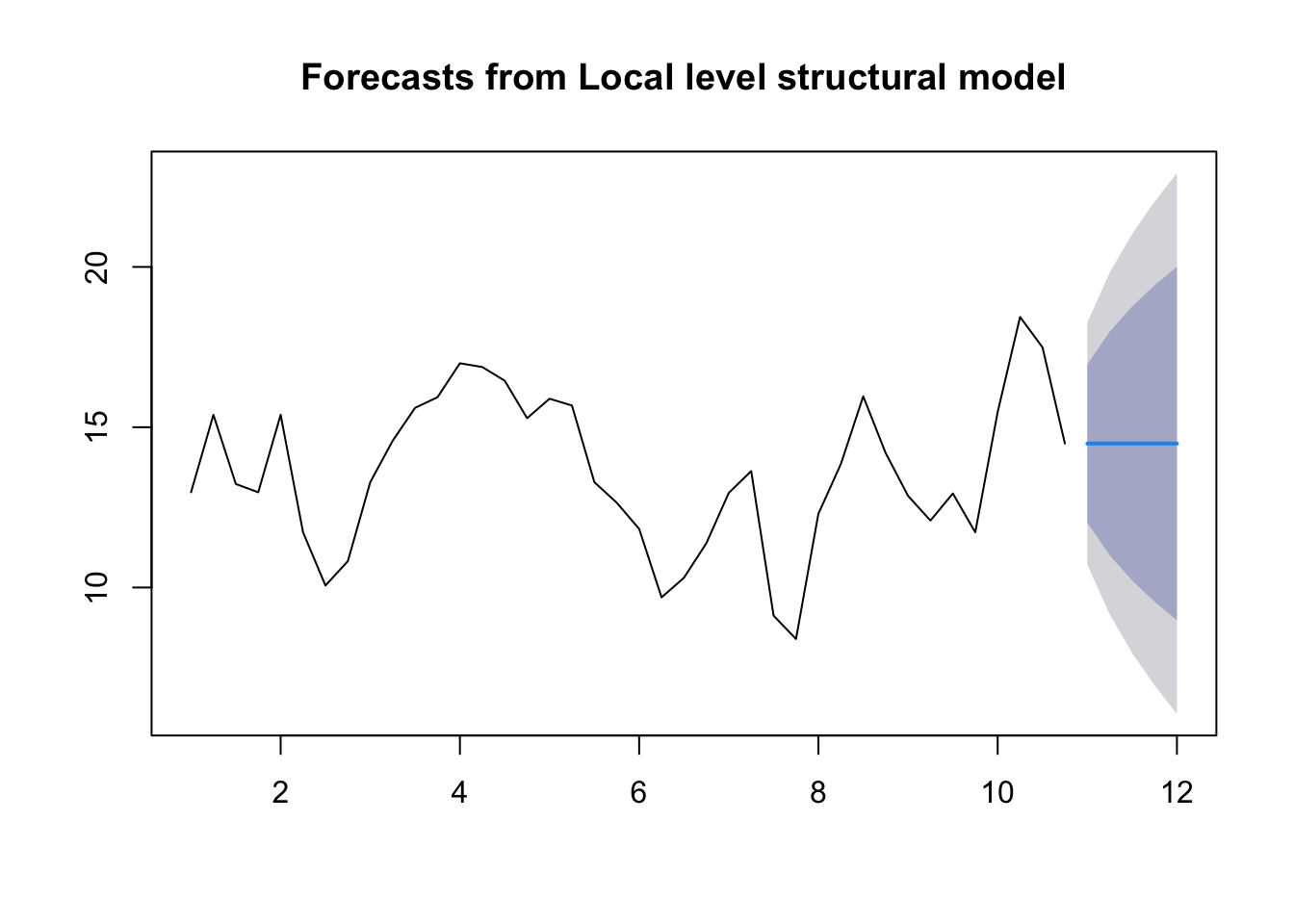
An alternate framework for time series modeling is the state space model. This model contains a lot of depth and flexibility. For additional model details, see this resource. These models are based on a decomposition of the series into a number of components, each of which may be accompanied by error terms (and thus, uncertainty). The simplest model is the local level model. In this model,
\[\begin{align} y_t &= \mu_t + \epsilon_t \\ \mu_t &= \mu_{t-1} + \tau_t. \end{align}\]
The idea of this model is that the observations \(y\) consist of noisy measurements (observation error) of an underlying random walk.
What is the estimate for \(\mu_t\) when \(\text{Var}(\tau_t) = 0\)? How about when \(\text{Var}(\epsilon_t) = 0\)? How does this relate to simple exponential smoothing?
6.4.2 Specific Problem
For the more general state space model we will use the package bsts.
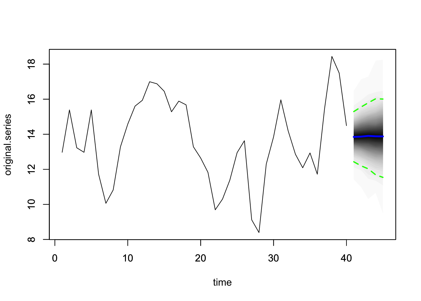
For our problem, we will introduce the covariate into the measurement equation. Our model is,
\[\begin{align} y_t &= \mu_t + \beta x_t + \epsilon_t \\ \mu_t &= \mu_{t-1} + \eta_t. \end{align}\]
We will use the package bsts to fit this model. The first thing to do when specifying a bsts package is the specify the contents of the latent state vector \(\mu_t\)
#library(bsts)
ss <- AddLocalLevel(list(), y)
model1 <- bsts(y ~ x1,
               state.specification = ss,
               niter = 1000)
## =-=-=-=-= Iteration 0 Tue Mar 5 15:17:25 2024 =-=-=-=-=
## =-=-=-=-= Iteration 100 Tue Mar 5 15:17:25 2024 =-=-=-=-=
## =-=-=-=-= Iteration 200 Tue Mar 5 15:17:25 2024 =-=-=-=-=
## =-=-=-=-= Iteration 300 Tue Mar 5 15:17:25 2024 =-=-=-=-=
## =-=-=-=-= Iteration 400 Tue Mar 5 15:17:25 2024 =-=-=-=-=
## =-=-=-=-= Iteration 500 Tue Mar 5 15:17:25 2024 =-=-=-=-=
## =-=-=-=-= Iteration 600 Tue Mar 5 15:17:25 2024 =-=-=-=-=
## =-=-=-=-= Iteration 700 Tue Mar 5 15:17:25 2024 =-=-=-=-=
## =-=-=-=-= Iteration 800 Tue Mar 5 15:17:25 2024 =-=-=-=-=
## =-=-=-=-= Iteration 900 Tue Mar 5 15:17:25 2024 =-=-=-=-=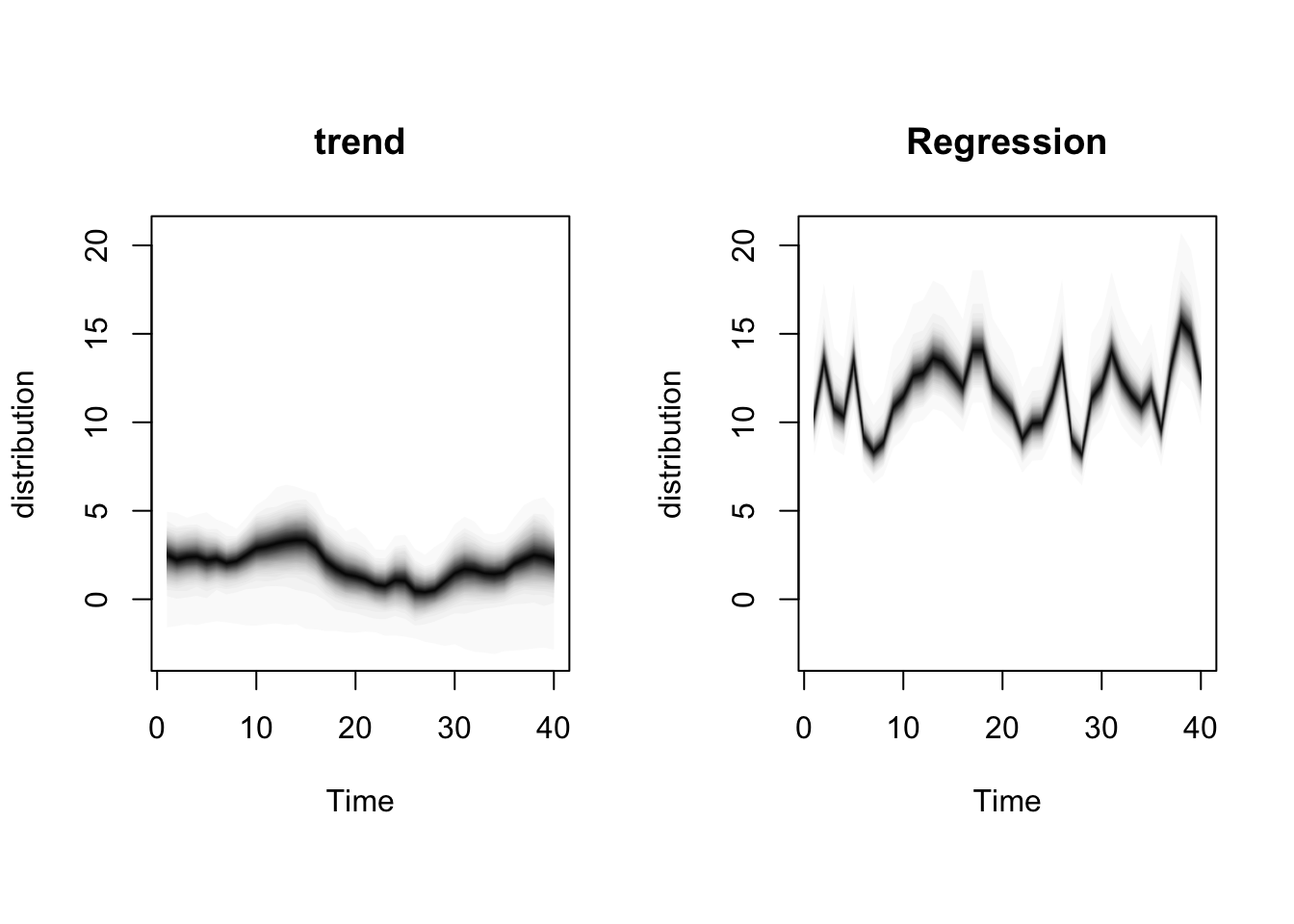
6.5 Lab 5
Suppose you are a commodities trader in Australia and you would like to model and forecast the demand for cattle (i.e., Cattle (excl. calves)) using the fpp3::aus_livestock dataset, using data from January 2017 through December 2018. Knowing the market for meat production in Australia, you plan to use the demand for bulls (i.e., Bulls, bullocks and steers) as a covariate in your models to make your forecasts more precise.
First, make a plot of these two time series (the total production per month across all States) starting in January 2017. Do they exhibit similar characteristics? What is the correlation between the two time series?
Fit a simple linear regression with cattle as the response variable and bulls as the predictor. What is the estimated model equation (i.e., the fit line equation)? Plot the residuals over time and the acf of the residuals. Do these plots indicate that any of the linear regression assumptions may be violated?
Using
dynlm, include a linear trend term in the linear regression from above (usingtrend), and include the first lag of bulls. Are the coefficients for these terms significant?Using
auto.arima, fit a linear regression with ARIMA errors using the same model setup as above (cattle as the response variable and bulls as the predictor). What is the model fit? Examine the residuals. Do they appear to be white noise?Using
bsts, fit a state space model with cattle as the response variable and bulls as the predictor (i.e., same model as Specific Problem). What is the estimated regression coefficient? How does this compare to the coefficient in the models fit above (i.e., question 2 and 4)? Make a plot of the model components.Of the three different model types with covariates (i.e., the linear regression fit in #2, the linear regression with AIRMA errors fit in #3, and the state space model fit in #5), which has the best performance? Make a table that shows the MSE for each model. For the second two model types, \(\hat{y}_t\) values can be obtained with the
predictfunction where you specify the covariate values using the observed values.